Bifurcations
Chaos
Fractals
Catastrophes
Self-organization
Emergence
Synchronization
Entropy
Agent-based modeling
Networks
Applications -- The Paradigm
Applications -- Psychology
Applications -- Biomedical
Applications -- Organizational Behavior
Applications -- Economics and Public Policy
Applications -- Ecology
Applications -- Education
Nonlinear Methods
Phase Space Analysis
Correlation Dimension
Surrogate Data and Experiments
Lypunov Exponent
Hurst Exponent
State Space Grids
Recurrence Plots and Analysis
Nonlinear Statistical Theory
Maximum Likelihood Methods
Markov Chains
Symbolic Dynamics
History of the BZ reaction produced by John A. Pojman.
Nonlinearity in Physics Tutorials by J. C. Sprott. Videotaped lectures explaining the basic principles of nonlinearity in physics.
|
Attractors
|
|
|
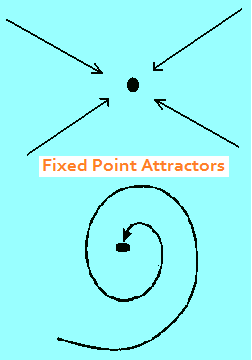
Attractors are the elements of nonlinear dynamics. An attractor is a piece of space. When an object enters, it does not exit unless a substantial force is applied to it. The simplest attractor is the fixed point. Some fixed points have spiral paths and some are more direct. Limit cycles and chaotic attractors are more complex in their movements over time, but they have the same level of structural stability. Structural stability means that all objects in the space are moving around according to the same rules.
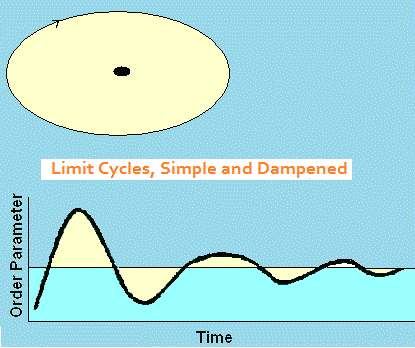
Oscillators, also known as limit cycles, are another type of attractor. Like the moon revolving around the early, once an object gets too close to the limit cycle it continues to orbit indefinitely or until a substantial force is applied. Oscillators can be pure and simple, or dampened to a fixed point by means of a control parameter. They can also be perturbed in the opposite direction to become aperiodic oscillators. There is a gradual transition from aperiodic produce a chaotic time series. A control parameter is similar to an independent variable in conventional research. Here it has the effect of altering the dynamics of the order parameter, which is similar in meaning to a dependent variable, except that it is not necessarily dependent. Order parameters within a system operate on their own intrinsic dynamics. Repellors are like attractors, but they work backwards. Objects that veer too close to them are pushed outward and can go anywhere, so long as they go away. This property of an indeterminable final outcome is what makes repellors unstable. Fixed points and oscillators, in contrast, are stable. Chaotic attractors (described below) are also stable in spite of their popular association with unpredictability. A saddle has mixed properties of an attractor and a repellor. Objects are drawn to it, but are pushed away once they arrive. An example is the perturbed pendulum shown at the right. A saddle is also unstable. |
   |
|
Bifurcations
|
|
|
Bifurcations are splits in a dynamic field that can occur when an
attractor changes from one type to another, or where different
dynamics are occurring in juxtaposing pieces of space. They
can even produce the appearance and disappearance of new
attractors. Bifurcations are patterns of instability that can be as
simple as a critical point, curved trajectories, or more complex in
structure. One or more control parameters is often involved to
change the system from one regime to the next.
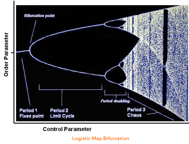
The logistic map is one of the classic bifurcations. It was first
introduced to solve a problem in population dynamics and has
seen a variety of applications since then. Start with the function
X2
= CX1 (1 - X1 ), with X1 and C in the range between 0 and 1.
Calculate X2 and run it through the equation again to produce X3, then
repeat a few more times. When C is
small, the results stay within a steady
state. When C becomes somewhat larger
(let it become gradually larger
than 1.0), X goes into oscillations.
As C becomes larger still, the
oscillations
become more complex (period doubling). When C = 3.6, the output is
chaotic.
The chaotic regime is rendered as a jumble of interlaced trajectories. The vertical striations are intentional. There are brief episodes of calm within the overal turmoil. Bifurcations are often experienced as critical points or tipping points. They are a critical feature of catastrophe models. |
|
Chaos Demonstrations by Clauswitz.com. Video clips and FLASH APPS for the Lorenz Attractor, Brownian Motion, 3- Body Problem, Double Pendulum, Perturbed Pendulum, Logistic Map and Bifurcation, The Game of Life, Complex Adaptive Systems, and more!
Nonlinear Dynamics and Chaos: A Lab Demonstration Stephen H. Strogatz. Video demonstrates various chaotic systems and applications: double pendulum, water flows, aircraft wing design, electronic signal processing, and chaotic music.
Lorenz Attractor in 3D Images by Paul Bourke.
Simple model of the Lorenz Attractor. [video]. Watch the attractor evolve and develop over time.
Interactive Lorenz Attractor by Malin Christersson. See the full range of Lorenz Attractor dynamics in 3D with this interactive display. Change parameters, or grab the image
|
Chaos
|
|
|
Chaos is a particular nonlinear dynamic wherein seemingly random events
are actually predictable from simple deterministic equations. Thus, a
phenomenon that appears unpredictable in the short term may indeed be
globally stable in the long term. It will exhibit clear boundaries and display
sensitivity to initial conditions. Small differences in initial states
eventually
compound to produce markedly different end states later on in time. The
latter property is also known as The Butterfly Effect and was first discovered
by Edward Lorenz during an investigation of weather patterns.
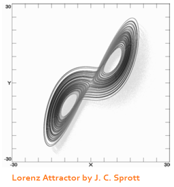
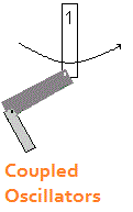
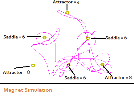
Chaos has some important connections and relationships to other dynamics, however, such as attractors, bifurcations, fractals, and self-organization. Not all examples of chaos are chaotic attractors, but several dozen structures for chaotic attractors are known, however. A chaotic attractor has the stability characteristic of the simpler attractors that were already described because all the points within the attractor and moving according to the same rule. The movements within the attractor basin are chaotic, and they contain both expanding and contracting movements. The paths of motion expend to the outer rim, then back again toward the center -- a pattern that can be observed in schools of fish or flocks of birds. The famous Lorenz attractor is shown at the right. A point moves along any of the trajectories on one lobe, but suddenly switches to the other lobe. The transition from one lobe to the other is as random as flipping a coin -- with the exception that it is a fully deterministic process instead. The Lorenz attractor is a system of three order paramters (movements along X, Y, and Z cartesean coordinates) and three control paramters. The control parameters goven the amount of spread between the lobes and their orientation along the cartesean axes. There are a few pathways by which a non-chaotic system can become chaotic. One is to induce bifurcations, an example of which was already described with the logistic map. Another pathway is to couple oscillators together. One oscillator acts as a control parameter that drives another oscillator. A third option is to create a field with multiple fixed point attractors close together and send an object into the field. The latter example actually captures the three body problem that Henri Poincare was studying in the 1890s when he first discovered what we call chaos today. The word chaos did not appear in the system science vocabulary until the 1970s, however. |
|
More About Fractals and Scaling by Larry Liebovitch. This online presentation covers some of the basic dynamical underpinnings of self-similarity.
The Mandelbrot Set by Malin Christersson. An iconic fractal that can be viewed at different levels of scale with this interactive display.
|
Fractals
|
|
|
A fractal is a geometric form in a non-integer number of dimensions, meaning that they do not fill up a whole 2-D or 3-D space. Fractals also have self-repeating structures. The same overall pattern is visible if we zoom in or out to different levels of scale. Their essential structures can be found in many examples in nature - the shapes of snowflakes, vegetable, lightning, neural structures. Why are they so visually engaging?
J. C. Sprott's Fractal of the Day website, shown at the right, changes every day at midnight, US Central Time. It deploys two basic algorithms. One selects a fractal structure, and the second evaluates the design for its level of complexity and other aesthetic properties. Please visit the archives, which can be reached by tracing the link. Fractal analysis can also be used to assess and compare the complexity of visual images such as abstract art works.
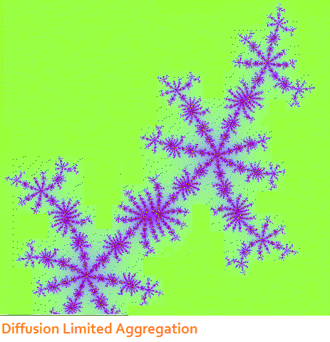
One of the more practical fractal functions is diffusion limited aggregation. This concept has been used to map the flow of contagious diseases across physical space. The pathogen spreads quickly down a central pathway, then fans out in multiple directions, then dissipates. The principle is more difficult to apply, however, when the pathogen spreads by means of a global transportation rather than simple physical proximity.
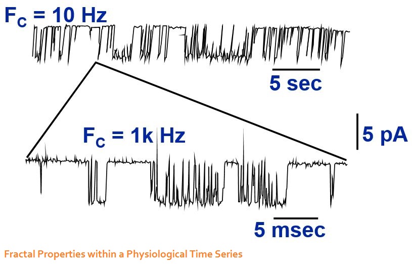
There is an important connection between fractal structure and chaos: The basin, or outer boundary of a chaotic attractor is a fractal. This discovery quickly led to the calculation of a fractal dimensions in time series data, which were in turn used to characterize the complexity of a time series of biometric or psychological data. In principle, it should be possible to find a fractal structure at one level of scale that repeats at other (finer, broader) levels of scale.
At one point in history, it was thought that the presence of a fractal structure in a time series was a clear indication that the time series was chaotic. This assumption turned out to be an oversimplification, however. A chaotic time series is composed of expanding and contracting segments. A much better "test for chaos" is the Lyapunov exponent associated with the time series.
A Lyapunov exponent is actually a spectrum of values that is computed from the sequential differences numbers in a time series. A positive exponent indicates expansion, and a negative value indicates contraction toward a fixed point. A perfect 0.0 indicates a pure oscillator, which, in practice could be a little bit perturbed in the chaotic direction or dampened in the direction of a fixed point. The decision about the dynamic character of a time series is drawn from the largest Lyapunov exponent, which should be positive, while the sum of the other values should be negative.
Conveniently, the largest Lyapunov exponent can be converted to a fractal dimension. Fractal dimensions between 0 and 1.0 indicate gravitation toward a fixed point. A value of 1.0 could indicate either a line or a perfect oscillator. Values between 1.0 and 2.0 are usually interpreted as the range of self-organized criticality, which reflects a balance between order and chaos. The connection between fractal structures, self-organization, and emergent events, which is developed later on in conjunction with self-organization.
Fractal dimensions between 2.0 and 3.0 are chaotic, but with a bias toward relatively small fluctuations over time that are perforated by a few large ones. An example would be the flight path of a bird of prey that is checking out its terrain suddenly swoops down to the group to check out something delicious. Humans adopt a similar pattern in a grocery store, probably without thinking about it. The caveat here, however, is that grocery stores are much more organized than the critters running through the woods. The grocery store wants us to find what we are looking for; the critters do not want to be found by the hawk.
Fractal dimensions greater than 3.0 are chaotic. One more caveat, however, is that there are many well-known chaotic attractors with fractal dimensions less than 3.0 and closer to 2.0. Not all examples of chaos are chaotic attractors.
|
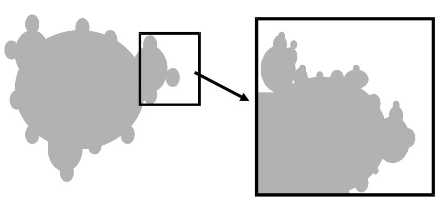
FRACTAL OF DAY LIVE FEED HERE Fractal of the Day
|
Catastrophe Machine prepared by the American Mathermatical Society, based on Zeeman's original.
|
Catastrophes
|
|
|
Catastrophes are sudden changes in events; they are not necessarily bad or unwanted events as the word "catastrophe" (in English) might suggest. Catastrophe models contain combinations of attractors, repellors, saddles, and bifurcations. According to the classification theorem developed by Rene Thom, all discontinuous changes of events can be described by one of seven elementary topological models. The models are hierarchical such that the simpler ones are embedded in the larger ones.
The simplest model is the fold catastrophe. It describe transitions
between a stable state (attractor) and an unstable state. The shift
between the two modalities is governed by one control parameter
(aka independent variable). When the value of that parameter reaches
a critical point, the system moves into the attractor state, or out of
it. Each catastrophe model contains a bifurcation set. In fold model,
the bifurcation set consists of a single critical point.
The catastrophe models are polynomial structures. The leading
polynomial for the fold response surface is a quadratic term, such
that f(y)/dy = y2 - a, in which a is the control parameter and y is the
observed behavior variable (aka, the dependent measure).
The catastrophe models also have a potential function, which char-
acterizes the behavior of agents that are acting within the model as
positions rather than velocities. In other words, to represent a velocity
we would say f(y)/dy or dy/dt (t = time). To represent the potential
function we would integrate the response surface function; thus for a
fold, f(y)= y3 - ay.
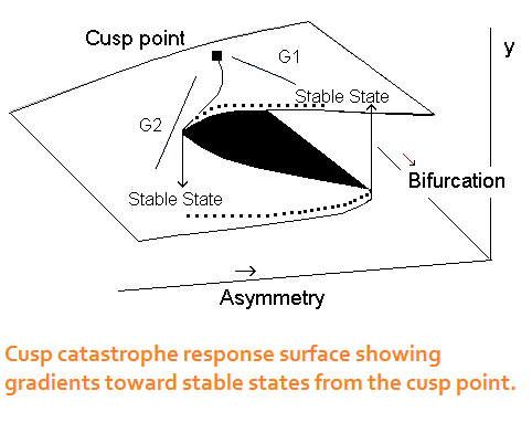
The cusp model is the second-simplest in the series - just complex
enough to be very interesting and uniquely useful. In fact it is over-
whelmingly the most popular catastrophe model in the behavioral
sciences. The cusp requires two control parameters, asymmetry and
bifurcation. To visualize the dynamics, start at the stable state on the
left and follow the outer rim of the surface where bifurcation is high.
If we change the value of the asymmetry parameter, nothing happens
until it reaches a critical point, at which we have a sudden change in
behavior: the control point that indicates what behavior is operating
flips to the upper sheet of the surface. A similar reverse process
occurs when shifting from the upper to the lower stable state.
When bifurcation is low, change is relatively smooth. The cusp point
is a saddle, and is the most instable location on the surface. With only a slight nudge it moves toward one of the
stable attractor states. The paths drawn in light blue are gradients that
are created by the two control variables. The red spot indicates the
presence of a repellor; comparatively few points land there.
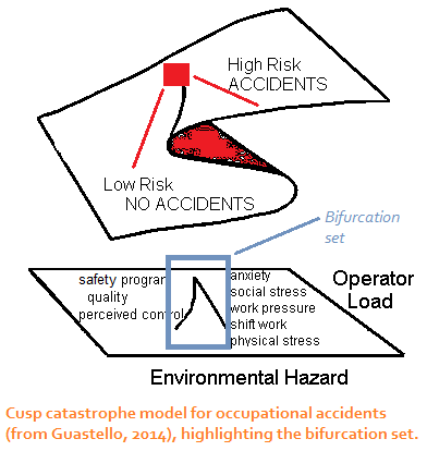
The cusp is often drawn with its bifurcation set, which is essentially a
2-dimensional shadow of the response surface. Therein you can see
the two gradients that are joined at a cusp point. In the application
to occupational accidents shown in the diagram, there were several psychosocial variables that contributed to the bifurcation parameter. Some had a
net-negative "influence" to them, and others had a positive "influence". Together the gradient variables capture the range of movements that are possible along the bifurcation manifold.
The leading polynomial
for the cusp response surface is a cubic term, such that f(y)/dy = y3
- by - a, in which a is the asymmetry parameter and b is the bifurcation
parameter. Its potential function is f(y) = y4 - by2 - ay.
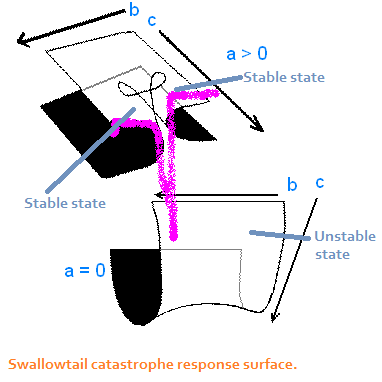
The swallowtail catastrophe model shows movement along a 4-
dimensional response surface that must be shown in two 3-D sections.
The leading polynomial for its response surface is a quartic polynomial:
f(y)/dy = y4 - cy2 - by - a. When the asymmetry parameter, a, is low
in value, objects on the surface can move from an unstable state to a
more interesting part of the surface (shown in the upper portion of the
figure to the right) where the stable states are located. The bifurcation
parameter, b, determines whether points will move from the back of
the surface to the front regions where the stable states are located.
Points can jump between the two stable states, or they can fall through
a cleavage in the surface back to the unstable state (low a). The bias
parameter, c, determines whether a point reaches one or the other stable
state.
The next four catastrophe models are more complex in structure, and thus have seen a lot fewer applications in the social sciences compared to cusps. Briefly, however, the butterfly
catastrophe describes movement along a 5-dimensional response
surface. It contains three stable states with repellors in between. Points
of objects can move between adjacent states in cusp-like fashion, or
between disparate states in a more complex fashion.
The model has four control parameters. The first three are asymmetry, bifurcations, and hears again. The fourth is the butterfly parameter which defeats the relationship between the hears and the bifurcation parameters.
The last three catastrophes belong to the umbilic catastrophe group.
They are distinguished by having 2 dependent measures (or order
parameters). The wave crest (or hyperbolic umbilic) model consists of
two fold-like variables that are controlled in part by the same bifurcation
parameter. Each behavior has its own asymmetry parameter.
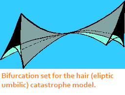
The hair (or eliptic umbilic) model has similar properties as the wave
crest, with the important addition that there is an interaction between
the two dependent variables. It gets its name from its bifurcation
set, which depicts three trajectories coming together at a hair-thin
intersection then fanning out again.The mushroom (or parabolic umbilic) model has one dependent measure
that follows cusp-like dynamics between two stable states and one
dependent measure that follows fold-like dynamics. The model contains
four control parameters, and there is an interaction between the two
dependent variables.
|
|
NK Rugged Landscape [PDF] -- a tutorial by Kevin Dooley
Please scroll down for more links and their accompanying narratives.
|
Self-Organization
|
|
|
A system that is in a state of chaos, high entropy, or far-from-equilibrium
conditions would exhibit high-dimensional changes in behavior patterns
over time, but not indefinitely so. Systems in that state tend to adopt new
structures that produce Self-organization is sometimes known as "order for
free" because systems acquire their patterns of behavior without any input
from outside sources.
There are four commonly acknowledged models of self-organization:
synergetics, introduced by Herman Haken; the rugged landscape, which
was introduced by Stuart Kauffman; the sandpile, introduced by Per Bak;
and multiple basin dynamics, introduced by James Crutchfield. What they
all have in common is that the system self-organizes in response to the
flow of information from one subsystem to another. In this regard the
principles build on the concepts of cybernetics that were introduced in the
early 1960s, and John von Neumann's principle of artificial life: all life can
be expressed as the flow of information.
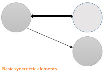
The basic synergetic building block is the driver-slave relationship, which
can be portrayed with simple circles and arrows. The driver behaves
over time (produces output or information) according to some temporal
dynamic such as an oscillation or chaos. The driver's output acts a control
parameter for to an adjacent subsystem, which one the one hand responds
to the temporal dynamics from the driver and produces its own temporal
output. In the simple case, the driver-slave relationship is unidirectional. In
other cases, such as when effective communication and coordination occur
between two people, the relationships are bidirectional.
A larger system would contain more circles and arrows. What we want to
know, however, is what do the arrows mean? This is where the dynamics
are of great importance.
Once patterns form and reduce internal entropy, the structures maintain
for a while until a perturbation of sufficient strength occurs that disrupts
the flow. The system adapts again to accommodate the nuances in some
fashion, either through small-scale and gradual change or a marked
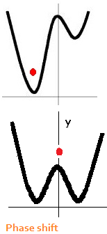
reorganization. The latter is a phase shift. For instance, a person might be
experiencing a medical or psychological pathology that is unfortunately
stable, and thus prone to continue, until there is an intervention. The intervention takes some time to be effective but the system eventually breaks up
its old form of organization and adopts a new one.
The phase shift in the
system is akin to water turning to ice or to vapor, or vice versa.
The
challenge is to predict when the change will occur. There is a sudden
burst of entropy in the system just before the change takes place, which
the researcher (therapist, manager) would want to measure and monitor.
A concise intervention at the critical point could have a large impact on what happens to the system next.
An important connection here is that the phase shift that occurs in
self-organizing phenomena is a cusp catastrophe function. Researchers
do not always describe it as such, but the equation they generally use
to depict the process is the potential function for the cusp; the only
difference is that sometimes the researchers hold the bifurcation variable
constant rather than a variable that is manipulated or measured.
The red ball in the phase shift diagram indicates the state the system is
in. In the top portion of the diagram it is stuck in a well that represents
an attractor. When sufficient energy or force is applied, the ball comes
out of the well and with just enough of a push moved into the second
well. In some situations we know what well we're stuck in, but not
necessarily what well we want to visit next. The question of how to form
a new attractor state is a challenge in its own right.
For the rugged landscape scenario, imagine that a species of organism
is located on the top of a mountain in a comfortable ecological niche.
The organisms have numerous individual differences in traits that are
not relevant to survival. Then one day something happens and the
organisms need to leave their old niche and find new ones on the
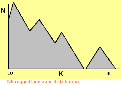
rugged landscape, so they do. In some niches, they only need one or
two traits to function effectively. For other possible niches, they need
several traits. As one might guess, there will be more organism living in a new 1-trait environment, not as many in a 2-trait environment, and so on. Figure 9 is a distribution of K, the number of traits required, and N the number of organisms exhibiting that many traits in the new environment. It is also interesting that there is a niche at the high-K end of the graph that seems to contain a large number of new inhabitants.
The niches in the landscape can also be depicted as having higher and lower elevation levels, where the highest elevation reflects high fitness for the inhabiting organism, and lower elevations for less fit locations. Organisms thus engage in some exploration strategies to search out better niches. Niches have higher elevations to the extent that there are many forms of interaction taking place among the organisms in the niche. The rugged landscape idea became a popular metaphor for business strategies in the 1990s. For further elaboration, see Kevin Dooley's linked contribution on rugged landscapes.
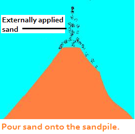
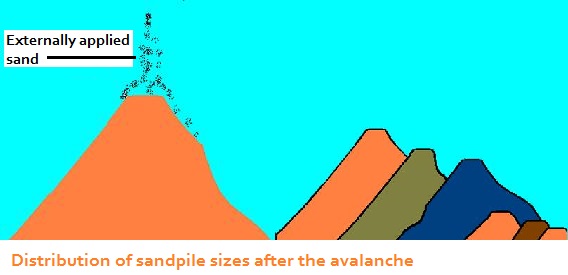
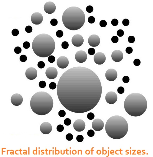
For the avalanche model, imagine that you have a pile of sand, and new sand is slowly drizzled on top the pile. At first nothing appears to be happening, but each grain of sand is interacting with adjacent grains of sand as new sands falls. There is a critical point at which the pile avalanches into a distribution large and small piles. The frequency distribution of large and small piles follow a power law distribution.
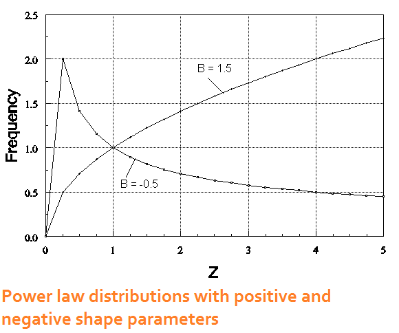
A power law distribution is defined as FREQ[X] = aXb, where X is the variable of interest (pile size), a is a scaling parameter, and b is a shape parameter. Two examples of power law distributions are shown in the diagram. Note the different shapes that are produced when b is negative compared to when b is positive. When b becomes more severely negative, the long tail of the distribution drops more sharply to the X axis. All the self-organizing phenomena of interest contain negative values of b. The |b| is the fractal dimension for the process that presumably produced them. The widespread nature of the 1/f/span> relationships led to the interpretation of fractal dimensions between 1.0 and 2.0 as being the range of self-organized criticality.
An easy way to determine the fractal structure of a self-organized process is to take the log of the frequency and plot it against the log of the object size. Then calculate a correlation between the two logs. The regression coefficient is the slope of the line, which is negative. The absolute value of the slope is the fractal dimension.
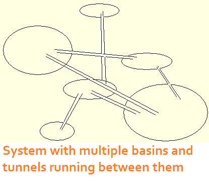
The multiple basin concept of self-organization also builds
on a biological niche metaphor and attempts to explain how
biological species could cross a species barrier. Imagine there
are several basins, each containing a population of some
sort. The populations stay in their niches while they interact,
change, and do whatever else they do. But the niches are
connected, so that once enough entropy builds up within a
basin, a few of the members bounce out into the adjacent
niche.
Multiple basin dynamics can also be found in economics
where, for instance, product designs and product prices
combine to meet distinct market needs. Sometimes, however,
a product producer will jump into another basin. It is an open
question as to how similar the process of jumping basins is to
jumping fitness peaks in the N|K model. Arguably, the multiple
basin scenario is a continuation of the N|K story.
|
|
|
Entropy
|
|
|
Entropy has been mentioned in conjunction with self-
organizing processes, but without definition until now. The
construct has undergone some important developments
since it was introduced in the late 19th century. In its first
incarnation it meant heat loss. This definition gave us the
principle that systems will eventually dissipate heat and
expire from "heat death." This generalization turned out to be
incorrect for a century later. When statistical physics gelled
in the early 20th century, entropy concerned the prediction
of the location of molecules in motion under conditions of
heat and pressure. It was not possible to target individual
molecules, but it was possible to create metrics for the
average motion of the molecules. This perspective
eventually led to the third incarnation, which was Shannon's entropy and
information functions in the late 1940s.
The Shannon metrics are probably the most widely used versions of entropy today, either directly or as a basis for the derivation of further entropy metrics. Imagine that a system can take on any of a number of discrete states over time. It takes information to predict those states, and any variability for which information is not available to predict is considered entropy. Entropy and information add up to HMAX, maximum information, which occurs when the states of a system all have equal probabilities of occurrence.
The nonlinear dynamical systems perspective on entropy, which is credited to Ilya Prigogine, however, is that entropy is generated by a system as it changes behavior over time, and thus it has become commonplace to treat information and entropy as the same thing and designate them with the same formula: Hs =  [p log2(1/p)], where p is the probability associated with an observation belonging to one category in a set of categories; the summation is over the set of categories. Some authors, however, continue to distinguish the constructs of information and entropy as they were originally intended.
Other measures of entropy have been developed for different types of NDS problems, however. A short list includes topological entropy, Kolmogorov-Sinai entropy, mutual entropy, approximate entropy, and Kullback-Leibler entropy and an associated statistic for the correspondence between a model and the data.
To return to self-organizing phenomena, self-organization occurs when the new structure provides a reduction in entropy associated with the possible alternative states of the system. In other words the system picks a state that it likes best, so to speak. The construct of minimum entropy, introduced by S. Lee Hong, or free energy, introduced by Karl Friston, reflect a system's proclivity to adopt a neurological, cognitive, or behavioral strategy that minimizes the number of degrees of freedom required to make a maximally adaptive response.
A related principle is the performance-variability paradox. There is a tendency to think of skilled performance (sports, music, carpentry) as actions produced exactly the same way each time they are produced. There are small amounts of variability, nonetheless, that arise from the numerous neurological and cognitive degrees of freedom that go into producing the action. You can prove the point to yourself by
signing your name six times on a piece of paper. Is each signature
exactly like the others? It is these degrees of freedom that make
an adaptive response and new levels of performance possible.
The complexity range of self-organized criticality reflects a
(living) system's balance between being complex enough to
adapt effectively and minimizing the number of free movements
necessary to do so. Unhealthy systems tend to be overly rigid.
Overly complex systems and behavioral repertoires tend to waste energy, which could be detrimental in other ways. [p log2(1/p)], where p is the probability associated with an observation belonging to one category in a set of categories; the summation is over the set of categories. Some authors, however, continue to distinguish the constructs of information and entropy as they were originally intended.
Other measures of entropy have been developed for different types of NDS problems, however. A short list includes topological entropy, Kolmogorov-Sinai entropy, mutual entropy, approximate entropy, and Kullback-Leibler entropy and an associated statistic for the correspondence between a model and the data.
To return to self-organizing phenomena, self-organization occurs when the new structure provides a reduction in entropy associated with the possible alternative states of the system. In other words the system picks a state that it likes best, so to speak. The construct of minimum entropy, introduced by S. Lee Hong, or free energy, introduced by Karl Friston, reflect a system's proclivity to adopt a neurological, cognitive, or behavioral strategy that minimizes the number of degrees of freedom required to make a maximally adaptive response.
A related principle is the performance-variability paradox. There is a tendency to think of skilled performance (sports, music, carpentry) as actions produced exactly the same way each time they are produced. There are small amounts of variability, nonetheless, that arise from the numerous neurological and cognitive degrees of freedom that go into producing the action. You can prove the point to yourself by
signing your name six times on a piece of paper. Is each signature
exactly like the others? It is these degrees of freedom that make
an adaptive response and new levels of performance possible.
The complexity range of self-organized criticality reflects a
(living) system's balance between being complex enough to
adapt effectively and minimizing the number of free movements
necessary to do so. Unhealthy systems tend to be overly rigid.
Overly complex systems and behavioral repertoires tend to waste energy, which could be detrimental in other ways.
|

|
SWARM Agent-based Modeling System -- Sante Fe Institute explains how the SWARM simulation system can be used to describe the self-organizing behavior of heatbugs, moustrap fission, and a small market with one commodity. Contains a portal to advanced materials for SWARM program users.
The Boids by Craig Reynolds. A simulation of a flock of birds developed by Craig Reynolds illustrates how a flock sticks together on the basis of only three rules. Other items on this site show similar properties for a school of fish, and reactions to predators or intruders. More swarms. More videos.
Santa Fe Institute's Complexity Explorer -- Online courses about tools used by scientists in many disciplies.
Evolving Cellular Automata Santa Fe Institute explains cellular automata as computational devices and system simulations for determining the results of self- organizing processes.
Emergence and complexity - Lecture by Robert Sapolsky [video]. He details how a small difference at one place in nature can have a huge effect on a system as time goes on. He calls this idea fractal magnification and applies it to many different systems that exist throughout nature.
|
Agent-Based Models
|
|
|
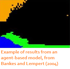
One of the problems that made the idea of complexity famous was that if many agents within a system are interacting simul- taneously, it is impossible to calculate the outcomes of each of them individually and predict further outcomes for other agents with which they interact. Calculating the possible orders in which they could possibly interact would be a daunting task by itself. What is possible, however, is to put the agents into a system and allow them to interact according to specific rules. We can also specify different rules for different agents, in which case we have heterogeneous agents. After the simulation has run long enough, the patterns of interaction stabilize into a self-organized system. The figure from Bankes and Lempert (2004) shows distribution of four types of entities that emerged after a period of time in which their agents interacted.
Agent-based models are part of a family of computational systems that illustrate self-organization dynamics such as cellular automata, genetic algorithms, and spin-glass models. Briefly, cellular automata are agent-based models that are organized on a grid. One cell affects the action of adjacent cells according to some specified rule. The example shown here is very elementary, but it conveys the core idea. The rule structures are chosen by the researchers within the context of a particular problem. The most extensive work in this area is credited to Stephen Wolfram and his New Kind of Science. Genetic algorithms were first developed to model real genetic and evolutionary processes without having to wait thousands of years to see results. An organism is defined as a string of numbers that represent its genetic code. Organisms then interact in a completely random fashion (or according to other rules specified by the researcher) and "breed." Mutation rules can also be coded into the system. New organisms are then tagged with a fitness index that defines their viability for survival. Ultimately we can see what happens to the computational species relatively soon. Genetic algorithms have also found a home in industrial design. For instance one can take two or more versions of an object, e.g. an automotive design, characterize them as a string of numbers, and let them breed. The results can be filtered for functionality and usability, and aesthetic properties. The winning possibilities might find their way into real-world production. Spin-glass models formed the basis of NK or Rugged Landscape models of self-organizing behavior. In principle some of the agents have common properties, and other agents have different common properties. The properties can be complex and defined and mixed up in any theoretically important way. After a certain amount of "spinning" together in a closed system, they aggregate into relatively homogeneous subgroups. To learn more about agent-based modeling and to see some examples in action, please visit some of the links included here. The Sugarscape model for artificial societies that was developed by economists at the Brookings Institute is particularly comprehensive for its logical development that closely parallels a real-world economy as rules of interaction are sequentially introduced. |
|
|
Emergence
|
|
|
The common use of the word has proliferated in recent years,
but it has a specific, technical origin. Psychologists remember
the maxim from Gestalt psychology, "The whole is greater than
the sum of its parts." The idea originated in scientific venues a
decade earlier, however, with the sociologist Durkheim, who was
trying to conceptualize the appropriate topics for a scientific study
of sociology. The central concern was that sociology needed to
study phenomena that could not be reduced to the psychology of
individuals. The essential solution went as follows: The process starts
with individuals who interact, do business, and so on. After enough interactions, patterns take hold that become institutionalized or
become institutions as we regularly think about them. When the
institution forms, it has a top-down effect on the individuals such
that any new individuals entering the system naturally conform
to the demands, and behavioral patterns, which are hopefully adaptive, of the overarching
system.
Emergence comes in two forms, light and strong. In the
light version, the overarching structure forms but does not have a
visible top-down effect. In the strong situations, there is a visible
top-down effect. The dynamics of emergence were captured in
some laboratory experiments by Karl Weick in the early 1970s
on the topic of "experimental cultures." Groups of 3 human
subjects were recruited for a group task. They worked together
until they mastered their routine. Then, one by one, the members
of the groups were replaced by a new person. The replacement
continued until all personnel were changed. At the end of 11
generations, the newest groups followed the same work patterns
as the original group, even though the originators were no longer
part of the system.
Two types of emergence are often observed in live social systems.
One is the phase shift dynamic. The second is the avalanche
dynamic that produces 1/fb relationships. Physical boundaries
have an impact on the emergence of phenomena as well.
Neuroscientists are also investigating the extent to which bottom-
up and top-down dynamics from brain circuits and localization
areas are combining to produce what is commonly interpreted as
"consciousness."
|
|
Synchronization
|
|
|
The first example of synchronization in mechanical systems was
reported in 1665 by Christiaan Huygens, who noticed that two
clocks that were ticking on their own cycles eventually ticked in
unison. The communication between clocks occurred because
vibrations were transferred between them through a wooden
shelf. Another prototype illustration is synchronization of a
particular species of fireflies, as told by Steven Strogatz: In the
early part of the evening the flies flash on and off, which is their
means of communicating with each other, which they do at their
own rates. As they start to interact, they pulse on and off in
synchrony so that the whole forest lights up and turns off as if one were flipping a light switch.
William Strutt opened investigations into the structure of sound waves in 1879, including those that appear synchronized. He observed that two organ pipes generating the same pitch and timbre would negate each other's sound if they were placed too close together. Thus two oscillators could exhibit an inverse synchronization relationship that he called oscillation quelching.
Based on the following century of advancements in the study of oscillating phenomena, Pikovsky et al. defined synchronization as "an adjustment of the rhythms of oscillating objects due to their weak interaction" (Synchronization: A universal concept in nonlinear sciences, 2001, p. 8). The oscillators must be independent, however; each one must be able to continue oscillating on its own when the others in the system are absent. Strogatz (Sync: The emerging science of spontaneous order, 2003) concisely described the minimum requirements for synchronization as two coupled oscillators, a feedback loop between them, and a control parameter that speeds up the oscillating process. When the control parameter speeds the oscillating process fast enough, the system exhibits phase lock.
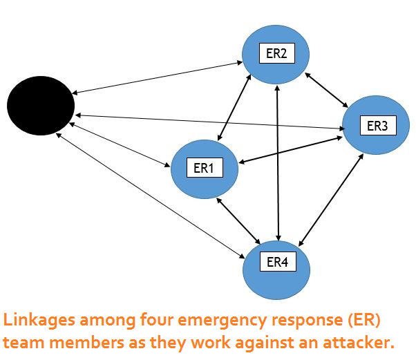
 Autonomic arousal levels (galvanic skin response) for four emergency response team members working against an attacker (GSR 5). Autonomic arousal levels (galvanic skin response) for four emergency response team members working against an attacker (GSR 5).In phase lock, the contributing oscillations all start and end at the same time, with start and end times varying only over a small and rigidly bounded range. If we imagine that the time series of observations produced by a pure oscillator is a sine wave and that its phase-space diagram is a circle, the positions of two or more synchronized oscillators are clustered together as they move around the circle at the same time. Phase synchronization is actually a matter of degree that depends on other matters of degree, such as the tightness or looseness of the coupling produced by the feedback, whether the feedback is unidirectional or bidirectional (or omnidirectional in the case of systems of multiple oscillators), and whether delays in feedback are prominent. The oscillators in a system are not restricted to pure forms; they can be forced, aperiodic, or chaotic processes. In fact, three coupled oscillators are sufficient to produce chaos. This principle has been exploited as a means for decomposing a potentially chaotic time series into its contributing oscillatory components. Chaos can also be controlled by imposing a strong oscillator on the system. Nervous systems are composed of many oscillating and chaotic subassemblies; some activate each other while others are inhibitory. Thus one would anticipate that the products of the nervous system - movements, autonomic arousal, speech and cognition patterns - are also fundamentally chaotic, and that pure oscillators are more often the exception than the rule. The journal Nonlinear Dynamics, Psychology and Life Sciences published a special issue on synchronization (April, 2016) that spanned synchronization within dyadic relationships, relationships that encompassed teams of four or six people, and finally the Nagent case (Sulis). The researchers asked questions such as who synchronizes to whom, in what way, and to what extent? What conditions affect the synchronization of movements, autonomic arousal, speech patterns, and brain waves? Principles of synchronization also lead to some pragmatic questions: How does synchronization promote more successful therapy sessions and more effective work teams? Are there conditions where synchronization is not in the best interest of the dyad or team? If synchronization, which often occurs at a nonverbal level of communication, contributes to desirable decisions and actions at a more explicit level, it can also facilitate negative emotions and irrationality, particularly if stressful conditions are involved. |
|
More about network structures and network analysis, by Matthew Denny, Institute for Social Science Research, University of Massachusetts, Amherst. [PDF]
|
Networks
|
|
|
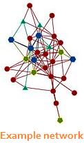
The idea of social networks was introduced by social psychologists
and sociologists in the early 1950s. Its underlying math comes from
graph theory. In the example diagram, the circles represent people,
and the arrows represent paths of communication, which can be
one-way or two-way. Network graphs are indifferent to the content
of the communication. People interact with each other about all
sorts of things - work, family and other social activities, common
interests, etc. In fact people interact about multiple common interests, so that one graph structure can be superimposed on
another.
More generally, the circles do not need to be people at all. They
can also be airports or other centers in a transportation network,
exchange points in a telephone system, or prey-predator relationships
within an ecological food web. The circles can also represent ideas
that come up frequently in conversations and become connected to
other ideas. Criminologists use network concepts to figure out who
is doing naughty things with whom. Marketing analysts use them to
figure out who is talking about their products and to figure out what
other products that people might like also. Ecologists use the same
constructs to assess the robustness and fragility of an ecosystem
when one of its contributing species is undergoing a sharp population
decline, perhaps due to human intervention.
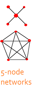
Networks can also be analyzed to determine the patterns of
communication that are needed to identify efficient and non-efficient alternative
configurations. For instance the star pattern of five people contains
a central hub that communicates with each of the other four
nodes, often bilaterally. The pentagon configuration, in contrast,
depicts five nodes that are communicating with all the other nodes
simultaneously, as in a group discussion.
One type of metric that can be applied to the analysis of networks
is centrality. There are three commonly used types of centrality:
degree, betweenness, and closeness. Degree is the total number of
links that a node can have relative to the total number of links in the
network. Betweenness is the extent to which a node gets in between
any two other connections. Closeness is the extent to which one node
connects to another with the smallest number of links in between.
Closeness is actually the inverse of degree, and people often like to
discuss how many degrees of separation exist between themselves
and somebody else (who might be famous).
As one might surmise, a node can become more central if it has
more links to the other entities in the network. If one were to assess
the frequency distribution of links associated with nodes within a network, the numbers of links are distributed as a 1/fb power law
function, with a small number of nodes having many links and
many nodes having much fewer links. The 1/fb nodes with the most
links become known as hubs in practical application. The pattern
strongly suggests (but does not necessarily prove by itself) that the
network is a result of a self-organizing process.
Studies of network structures, primarily due to Albert Barabasi,
Duncan Watts, and Steven Strogatz, uncovered some interesting
and useful properties of random, egalitarian, and small-world
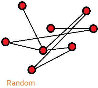
networks. A random network is just what its name implies: A group
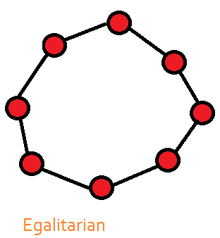
of potential nodes is connected on a random basis. An egalitarian
network is one in which each node communicates to its two next-
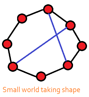
door neighbors, but no further. If we were to drop a random
connection into either type of network, the average number of
degrees between any two nodes drops sharply. Hubs start to form,
and we end up with a small-world network in which the average
number of degrees between nodes is approximately 6. Thus, in a
small world, anyone can reach, or be connected to, anyone else in
six links or less; the challenge, however, is to figure out which six
links will do the job.
The robustness of system architectures has numerous practical
implications. If a small world is subject to a random attack, meaning
that the attack is against one node selected at random, the network
will survive because there are enough communication pathways
to link the remaining nodes to each other. If a hub is attacked, the
survival of the network could be in big trouble.
The foregoing dynamics depict how a network could self-organize
into a 1/fb distribution of connections that produce hubs. Hubs
become attractors in the sense that they attract more connections:
people move to cities, airlines organize their routes around
hub airports, and so on. The avalanche dynamic looms in the
background, however: Physical systems have a limit to their carrying
capacity. Cities become congested and polluted and airports
struggle to maintain flight schedules and proper air traffic control.
One can probably think of more examples. When the carrying capacity is reached, it becomes advantageous to move out of the city, find a new airport to grow, or adapt one's occupation to one that has less competition for resources and attention. The big hub breaks into smaller units that are more equal in size. Per Bak showed, however, that the avalanche produces smaller sand piles that are distributed 1/fb in size. Thus the process is likely to repeat in some fashion.
So far we have focused on the nature of the nodes, but what about the connections? The distinction between strong versus weak ties that has some important dynamical implications. In human communication, strong ties mean rapid dissemination of information within the network. As a result there is a rapid uptake of ideas, which can be convenient many times. The limitation is that the importation of new information becomes unlikely. In those situations, weak ties with other nodes offer the benefit of reaching out to many more nodes, albeit less often, to collect new informational elements.
In a food chain, a predator-prey relationship in which the predator only eats one or a very few specific prey is a strong tie. If an ecological disaster compromises the prey population, the predator is in similar trouble. If the predator has more omnivorous tastes, and thus has weak ties to any one particular food source, the predator can leverage itself against a loss of a tasty favorite and survive.
|
|
This special issue of Nonlinear Dynamics, Psychology, and Life Sciences (January, 2007) was devoted to the paradigm question as it was manifest in a variety of disciplinary areas. See contents. Inquire about availability.
The Impact of Edward Lorenz. Special issue of NDPLS (July, 2009) pays a historical tribute to Lorenz discovery of the butterfly effect, its mathematical history, later developments, and its applications in economics, psychology, ecology, and elsewhere. See contents. Special order this issue.
The Nonlinear Dynamical Bookshelf is a regular feature of the SCTPLS Newsletter (sent to active members) that presents announcements and brief summaries of new books on topics related to nonlinear dynamics. Contents are limited to information we can collect from book publishers or that crawl into our hands by any other means.
Open access book reviews: In an effort to help the world get caught up on its reading, NDPLS has made its book reviews published since 2004 free access on its web site. Browse the journal's contents to see the possibilities.
Books written by members of the Society for Chaos Theory in Psychology & Life Sciences. This list is as complete as we can get it for now, and it is updated regularly. Most are technical in nature. Some of these works go beyond the scope of nonlinear science. Some are whimsical. All are recommended reads.
Recent books by members is a sub-list of the above that lists only those books published with in the past four years.
|
Applications - The Paradigm
|
|
|
There are many applications of nonlinear dynamics in psychology, biomedical sciences, sociology, political science, organizational behavior and management, macro- and micro-economics. We can only provide an overview here and direct our readers to more resources using the links on the panel to the left.
So let's start with the big picture - the paradigm. Nonlinear theory introduces new concepts to psychology for understanding change, new questions that can be asked, and offers new explanations for phenomena. It would be correct to call chaos and complexity theory in psychology a new paradigm in scientific thought generally, and psychological thought specifically. A special issue of Nonlinear Dynamics, Psychology, and Life Sciences in January, 2007 was devoted to the paradigm question, which actually spans across the various disciplines we study. The highlights of the paradigm are:
1. Events that are apparently random can actually be produced by simple deterministic functions; the challenge is to find the functions. 2. The analysis of variability is at least as important as the analysis of means, which pervades the linear paradigm. 3. There are many types of change that systems can produce, not just one; hence we have all the different modeling concepts that have been described thus far. 4. Contrary to common belief, many types of systems are not simply resting in equilibrium unless perturbed by a force outside the system; rather, stabilities, instabilities, and other change dynamics are produced by the system as it behaves "normally." 5. Many problems that we would like to solve cannot be traced to single underlying causes; rather, they are product of complex system behaviors. 6. Because of the above, we can ask many new types of research questions and need to develop appropriate research methods for answering those questions. Such efforts are well underway (see further along on this Resources page). Nonlinear science is an interdisciplinary adventure. Its growth has been facilitated by the interactions among scientific disciplines, as they are traditionally defined. Scientists soon discover that there are common principles the underlie phenomena that are seemingly unrelated. Consider some quick and blatant examples: 1. The phase shifts that are associated with water turning to ice or vapor follow the same dynamical principles as the transformations made by clinical psychology patients from the time of starting therapy to the time when the benefits of therapy are realized in their lives. 2. The changes in work performance (or error rates) as a person's mental workload becomes too great follows the same dynamics as the buckling of a beam, the materials for which could range from elastic and flexible to rigid and stiff. 3. The growth of a discussion group on the internet parallels that of a population of organisms, which is limited by its birth rate and environmental carrying capacity. 4. The transformation of a work team from a leaderless group into one with primary and secondary leadership roles as its task unfolds bears a close resemblance to the process of speciation in Kauffman's NK[C] model as an organism finds new ecological niches in a rugged landscape. (The former is a less complex version of the latter, however.) |
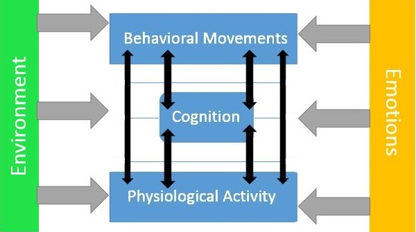 The most recent perspective in
psychology generally might be
termed 'the biopsychosocial
answer to everything.' Researchers
are looking for patterns and
connections between physiological
activity (patterns in EEGs or autonomic arousal), cognition, and
obvious behaviors. Emotions and the
environment affect all three major
domains. The opportunities for
nonlinear dynamics are abundant.
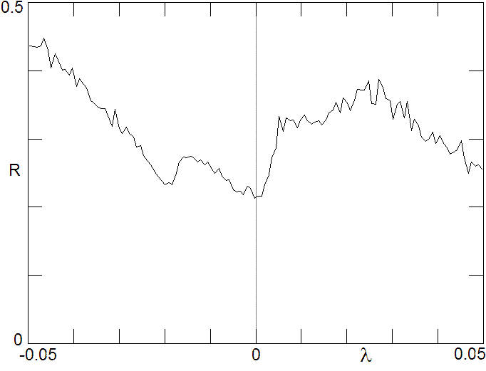 Research Example 1: Average learning
rate as a function of the Lyapunov
exponent showing that weak chaos
(positive
  ) is beneficial for learning
in this artificial neural network. From
Sprott, J. C. (2013). Is chaos good for
learning? NDPLS, 17(2), 223-232. ) is beneficial for learning
in this artificial neural network. From
Sprott, J. C. (2013). Is chaos good for
learning? NDPLS, 17(2), 223-232.
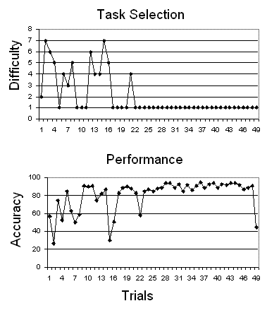 Research Example 2: Time series for task selection and performance for one participant in a multitasking study who used the 'favorite task' strategy. From Guastello et al. (2013). The minimum entropy principle and task performance. NDPLS, 17(3), 405-424.
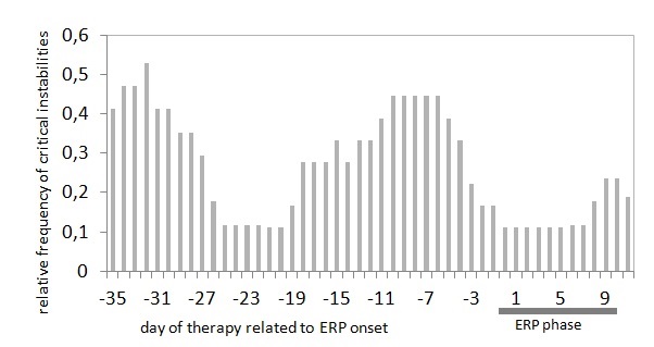 Research Example 3: Relative frequency
of critical instability periods
during psychotherapy. Two phases
can be identified where the relative
frequencies of critical stabilities
increases above 40%, which occur at
the beginning of the therapy and in
the phase before exposure-response
prevention (ERP). From Heinzel,
S., Tominschek, I., & Schiepek,
G. (2014). Dynamic patterns in
psychotherapy: Discontinuous
changes and critical instabilities
during the treatment of obsessive
compulsive disorder. NDPLS, 18(2),
155-176.
|
Article: "Chaos as a Psychological Construct: Historical Roots, Principal Findings, and Current Growth Directions" by S. J. Guastello
Chaos, Complexity, and Creative Behavior. Special issue of NDPLS (April, 2011) explores nonlinear dynamics of the cognitive, process, product, and diffusion aspects of creative behavior. See contents. Inquire about availability.
Developmental Psychopathology. Special issue of NDPLS (July, 2012) examines parent-child interactions from a dynamical point of view. See Contents. Inquire about availability.
Interpersonal Synchronization. Special issue of NDPLS (April, 2016) examines a fast-moving research area about how body movements, autonomic arousal, and EEGs synchronize between dyads, such as therapy-client dyads, and larger work teams, and the effect synchronization has on various outcomes. See contents. Special order this issue.
Article: "Nonlinear Dynamics in Psychology" by S. J. Guastello. This open access article from Discrete Dynamics in Nature and Society, vol. 6, pp. 11-29, 2001 gives an overview of applications in psychology, except neuroscience, as they existed through early 2000.
|
Applications - Psychology
|
|
|
Psychology has been transforming rapidly with the nonlinear influence. Applications of NDS in psychology include neuroscience; psychophysics, sensation, perception and cognition; motivation and emotion, group dynamics, leadership, and collective intelligence; developmental, abnormal psychology and psychotherapy; and organizational behavior and social networks. The Society's book project, Chaos and Complexity in Psychology: The Theory of Nonlinear Dynamical Systems provides a state-of-the-science compendium (through 2008) of psychological research on the foregoing topics in textbook format. The chapter authors make frequent contrasts between the conventional scientific paradigm and the nonlinear paradigm.
The article that follows in the list of links, "Chaos as a Psychological Construct" examines the concept of chaos as it has appeared in a wide range of psychological literature. Uses of the construct range from common use of the word chaos, which usually has no intended reference to formal nonlinear dynamics, to applications where chaos is meant seriously. The research efforts that follow on this page, in psychology and elsewhere, use NDS constructs literally and analytically.
The resources list for psychology includes special issues of Nonlinear Dynamics, Psychology, and Life Sciences that are focused on psychomotor coordination and control, creativity, brain connectivity, developmental psychopathology, organizational behavior, and education, and interpersonal synchronization. Other special issues are in the works, and announcements of new projects will appear on our NEWS page and the NDPLS home page. To make matters more interesting, many areas of psychology have embarked on the "biopsychosocial explanation of everything." There is a growing awareness of the interconnections among brain and nervous system activity, cognitive processes and social processes now that we are learning much more about all three realms. The opportunities for new works - and stronger explanations for phenomena - in nonlinear dynamics are extensive. Consider what else is going in the biomedical sciences (next). |
Medical Practice. Special issue of NDPLS (October, 2010) offers theoretical and empirical studies that indicate that a paradigm shift in neurology, cardiology, rehabilitation, and other areas of medical practice is very necessary. See contents. Special order this issue.
Brain Dynamics. Special issue of NDPLS (January, 2012) explores developments in brain connectivity and networks as seen through temporal dynamics. See contents. Special order this issue.
Neurodynamics: Special issue of NDPLS in honor of Walter J. Freeman III. Contributing authors extend Freeman�s progressive thinking to new frontiers. See contents. Editorial introduction. Special order this issue.
Psychomotor Coordination and Control. Special issue of NDPLS (Jan. 2009) explores developments in psychomotor learning and skill acquisition and applications to rehabilitation. See contents. Special order this issue.
Handbook on Complexity in Health, edited by J. P. Sturmberg & C. M. Martin (2013) offers over 1000 pages of viewpoints and research on medical thinking and practice, behavioral medicine and psychiatry from the perspective of nonlinear dynamics and complex systems. See table of contents.
|
Applications - Biomedical Sciences
|
|
|
Some of the first applications in the biomedical sciences explored the comparisons of the fractal dimensions of healthy and unhealthy hearts, lungs, and other organs. Larger dimensions, which indicate greater complexity, were observed for the healthy specimens. This finding gave rise to the concept of a complex adaptive system in other living and social systems. In the area of cognitive neuroscience, memory is now viewed as a distributed process that involves many relatively small groupings of neurons, and that the temporal patterns of neuron firing contain a substantial amount of information about memory storage processing. The temporal dynamics of memory experiments can elucidate how the response to one experimental trial would impact on subsequent responses and provide information on the cue encoding, retrieval, and decision processes. One might examine behavioral response times and rates, the transfer of local electroencephalogram (EEG) field potentials, similar local transfers in functional magnetic resonance images. In light of the complex relationships that must exist in processes that are driven by both bottom-up and top-down dynamics, the meso-level neuronal circuitry has become a new focus of attention from the perspective of nonlinear dynamics.
Dynamical diseases, which were first identified by Leon Glass, are those in which the symptoms come and go on an irregular basis. As such, the underlying disorder can be difficult to identify and the symptoms can be difficult to control unless one reframes the problem as one arising from the behavior of a complex adaptive system. This notion has now carried over to the analysis of psychopathologies with some success. There are, in turn, further implications for medical practice, David Katerndahl and other writers have observed that the mainstay of medical practice in most countries still revolves around the single cause mentality.
|
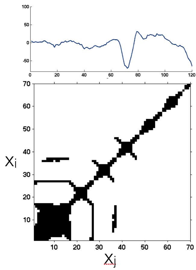 Research Example 4: A sample
EMG time series and corresponding
recurrence plot for one participant
during a single experimental trial of a
vertical jump task. From Kiefer, A. W.,
& Myer, G. D. (2015). Training the antifragile
athlete: A preliminary analysis
of neuromuscular training effects on
muscle activation dynamics. NDPLS,
19(4), 489-510.
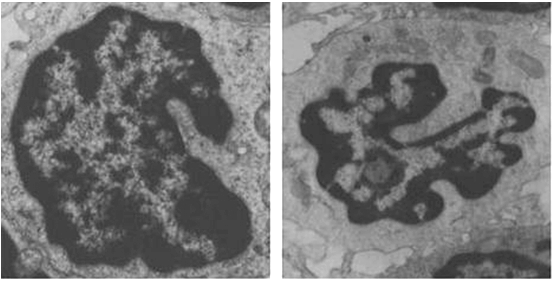 Research Example 5: The shape of the
T cells nuclei (transmission electron
microscopy of the skin, x 15000) is
more complex in the tumor (right)
in comparison to flogosis (chronic
dermatitis, left). From Bianciardi, G.
(2015). Differential diagnosis: Shape
and function, fractal tools in the
pathology lab. NDPLS, 19(4), 437-464.
|
Article: "A Complex Adaptive Systems Model of Organizational Change," by K. J. Dooley.
Article: "Nonlinear dynamical systems for theory and research in ergonomics," by S. J. Guastello. Ergonomics, 2017, 60, 167-193. Request reprint from author.
Advanced Modeling Methods for Studying Individual Differences and Dynamics in Organizations. In this special issue of NDPLS, authors consider the possible uses of growth curve modeling, agent-based modeling, cluster analysis, and other techniques to explore nonlinear dynamics in organizations. See Contents. Editorial introduction. Special order this issue.|
Applications - Organizational Behavior
|
|
|
Organizational Behavior grew up from a combination of influences, most of which stem from Industrial/Organizational Psychology, although there are important influences from other areas of psychology, sociology, cultural anthropology, contemporary management, and economics. In short, it is the study of people at work. The subject area had undergone roughly five paradigm shifts over the last century while trying to answer just one question, "What is an organization?"
1. During the rise of large corporations in the late 19th century there was no answer. Business organizations were managed on an ad hoc basis, which is to say the opportunities for chaos and confusion in the conventional sense abounded and intuition prevailed. Organizational leaders had few role models other than the military and the Catholic Church, both of which were command-and-control structures then and not much different now.
2. Weber, a sociologist introduced the concept of bureaucracy circa 1915, which was intended to instill rationality and efficiency where there was none before. People were separate from their roles. It was the roles that had rights and responsibilities. The drive toward impersonality and supposed efficiency had a negative consequence, which was to produce impersonal and mechanistic enterprises with people being plug and play machine parts.
3. The nature of organizations changed drastically with the introduction of humanistic psychology, which extended not only to the understanding of individual personality, but the role of people in organizations. The full capabilities of an organization could be unleashed by giving the normal human tendencies to grow and achieve new opportunities for expression. Here entered psychologist Kurt Lewin, whose platform work on organizational change (a.k.a. organizational development) facilitated the first understanding of social change and intervention processes. Most of the early change efforts were directed at changing an organization from a mechanistic and authoritarian bureaucracy to an enterprise that was consistent with human nature.
4. The transition to the organic model was not as dramatic as the previous change in viewpoints. The new understand was, nonetheless, that the organization itself is a living entity, and not simply humans in a nonliving shell. Organizational life bore many similarities to the biological life of single organisms. The organic model was an important step along the way to what came next.
5. The current paradigm, and answer to the question, "What is an organization" is: A complex adaptive system. Here we can observe all the principles of nonlinear dynamics - chaos, catastrophe, self-organization and more - occurring in relationships between people and their work, the functionalities of work groups, work group dynamics, the relationship between the organization and its environment and organizational change. This line of thinking has broad implications for leadership before, during, and after an organizational change process. In fact, change is now understood to be ongoing and business as usual, and not confined to deliberate interventions. Deliberate interventions are often necessary none the less.
The new paradigm is explicated in "A Complex Adaptive Systems Model of Organizational Change," by K. J. Dooley. The article debuted in the inaugural issue of NDPLS in 1997, and remains a landmark in our new understanding of organizational behavior.
Organizational behavior, or I/O Psychology, was among the first application areas of NDS in psychology, with the first contributions dating to the early 1980s. Extensive work on organizational theory has followed since then.
Human factors (engineering) started as the psychology of person-machine interaction - everything that took place at the interface between person and machine. There was also some concern with the interface between the person and the immediate physical environment. The psychological part of the subject matter is primarily cognitive in nature. The area has merged in scope with ergonomics, which started with interaction between people and their physical environment and numerous tpoics in biomechanics.
In light of new technological transitions and the growth in connected networks of people and machines, human factors and ergonomics have expanded further to include group dynamics regularly, and organization-wide behavior in some of the most recent efforts. Of particular importance here, there is now a further recognition of systems changing over time and the nonlinear dynamics involved, such that it is now possible to define NDS as a paradigm of human factors and ergonomics. Applications of particular interest include nonlinear psychophysics where the stimulus source and observer are in motion, control theory, cognitive workload and fatigue, biomechanics connected to possible back injuries, occupational accidents, resilience engineering, and work team coordination and synchronization.
|
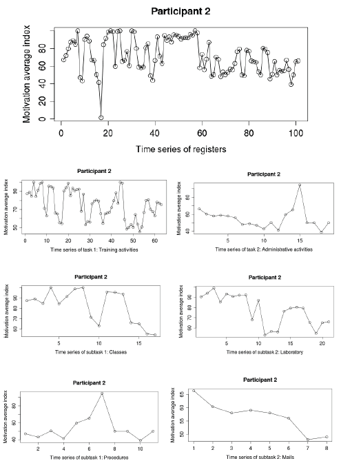 Research Example 6: Line chart of
work motivation fluctuations across
different scales: work tasks and
subtasks for one participant. From
Navarro, J. et al. (2013). Fluctuations
in work motivation: Tasks do not
matter! NDPLS, 17(1), 3-22.
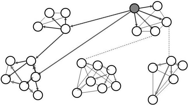 Research Example 7: Cooperating
units form capabilities. Multi-agents
that cooperate through leadership
influence converge toward attractors.
Agent to agent influence is based
on perceived 'reputation' while
competition to connect to the most
centralized agents consolidates
influence in 'leader roles' shown in
gray. From Hazy, J. (2008). Toward
a theory of leadership in complex
systems: Computation modeling
explorations. NDPLS, 12(3), 281-310.
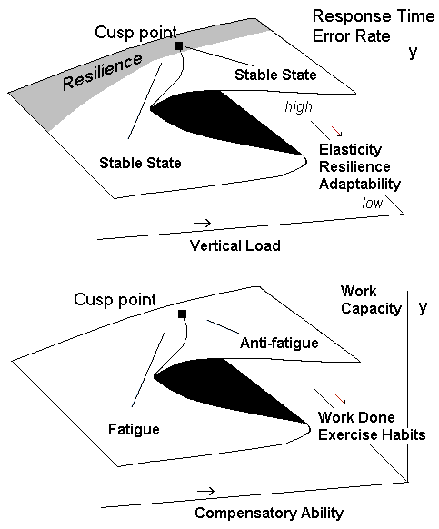 Research Example 8: Cusp catastrophe
models for cognitive workload and
fatigue. Both processes are thought to
be operating simultaneously during
task performance. From Guastello, S. J.,
et al. (2013). Cusp catastrophe models
for cognitive workload and fatigue: A
comparison of seven task types. NDPLS,
17(1), 23-48.
|
Article: "Complexity and Behavioral Economics" by J. B. Rosser, Jr. & M. V. Rosser (2015). The works of H. Simon figure prominently in this survey-review article.
|
Applications - Economics & Policy Sciences
|
|
|
The relationship between concepts from economics and physics, nonlinear and otherwise, dates back to the early 20th century. The Walrasian equilibrium established what is now the 'conventional' of 'classical' paradigm in economics which posits that the economy is an a natural equilibrium state (something akin to 'homeostasis'), which is most often assumed to be a fixed point, unless it is perturbed by agents or events from outside the immediate system. The study of business cycles, however, changed the view of what an 'equilibrium' could really mean, and once connections between the cycles were established, it became clear that chaos was possible. Variations in system behavior (e.g., securities prices, unemployment, inflation) could no longer be attributed to influences from outside; they needed to be interpreted as the natural dynamics of the system and that the natural or intrinsic dynamics could generate much more than fixed points. For more about the contrast between the classical and nonlinear paradigms, please see the article by Dore and Rosser that is linked in the left column.
The Nash equilibrium which evolved into game theory, is another notable example. Game theory became a key concept in psychological, economic, and other agent-based dynamics since that time. The advent of evolutionary game theory in the early 1980s particularly the work of Robert Axtell and John Maynard Smith extended the reach of nonlinear simulation studies. Evolutionarily stable states, which developed from thousands of agents playing the same game, have some connection to the equilibria formed by any two individual agents, but could be substantially different from the individual-level equilibria. What we are actually seeing is a global structure emerging from the interactions among individual agents. Rosser's 3-volume set (Menu 3) compiles the critical work in nonlinear economics that appeared in many journals through 2004. Even more has happened since then. Finance is one of four broad areas of economics that is replete with nonlinear dynamics. Macroeconomics is another challenging dynamical domain. Some schools of economic thought attempt to reduce system-level events to the decisions of individual financial agents. NDS studies in macroeconomics, however, are more consistent with other schools of economic thought that assume that one cannot assume a particular system-level outcomes, such as inflation or unemployment from knowledge of forces acting on individual economic agents. Ecology is another active area of nonlinear science. The discovery of the logistic map function actually arose in the context of population dynamics, and birth rates and environmental carrying capability change.
Ecological economics is a third broad area that lends itself to NDS analysis. Topics in this group include environmental resource protection and utilization, agricultural management, and land use and the fractal growth of urban areas. Cellular automata have been useful tools for studying urban expansion, as one example.
Evolutionary economics is the study of behavior change on the part of microeconomic agents, institutions, or macroeconomic structures. Here one finds chaos and elementary dynamics, game-theoretical experiments with evolutionary stable states, and multi-agent simulations based on genetic algorithms or other computational strategies grounded in NDS theory. An important part of policy making in any of these area is the ability of the decision makers to recognize the "time signatures" of various dynamical processes and plan accordingly. The efficacy of the current wave of institutional policymakers for doing is an open question. In fact, real-world events often involve dynamics that occur on several temporal time horizons. In the case of response to natural disasters for instance, there is long-term planning for the possibilities, shorter-term response when an earthquake or tsunami actually happens, and responses that occur in the scale of minutes and seconds when people need to act in the moment to save a life. We recommend the article on time ecologies by Gus Koehler, which appears in the list of links. |
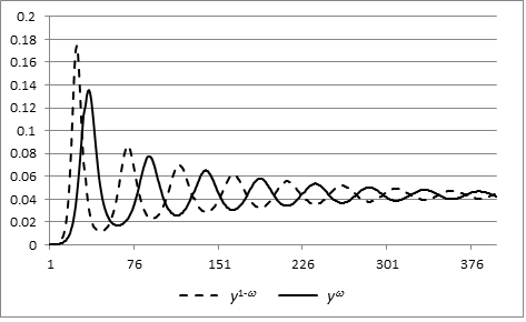 Research Example 9: Densities of
exuberant optimists and exuberant
pessimists in market activity as time
unfolds. From Gomes, O. (2015). A
model of animal spirits via sentiment
spreading. NDPLS, 19(3), 313-343.
|
|
Applications - Ecology
|
|
|
Ecological applications of NDS fall into the domains of both biologists
and economists. Topics of nonlinear interest most often include
population dynamics, prey-predator dynamics, the complex web
of relationships among co-dependent species, and the impact of
human interventions such as fish and livestock harvesting and
agriculture generally.
The logistic map function, which was described above as a classic
bifurcation structure, originated with population studies, and has in turn inspired numerous studies outside of ecology that involve
transitions between chaotic and non-chaotic temporal patterns.
Robert May is credited for landmark modeling strategies for ecological systems that involve birth
rates, environmental carrying capacity, and other intervening
factors.
|
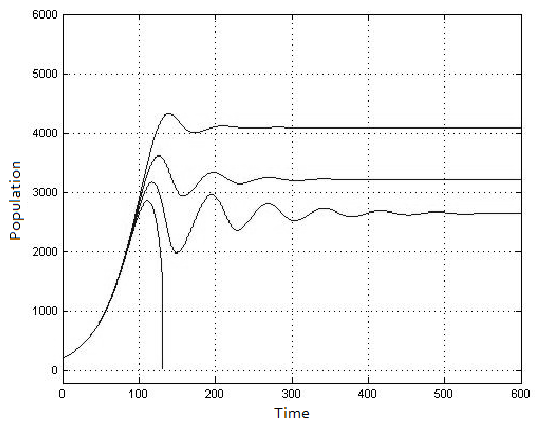 Research Example 10: The human
population of Easter Island is graphed
for f (decrease in the growth rate of
trees) ranging from .0004 to .001.
For small values of f the population
oscillates around the coexistence
equilibrium, and for larger values of
f the human population is unstable
and crashes. These diagrams illustrate
that the stability of the coexistence
equilibrium in the Invasive Species
Model is sensitive to the parameter
modeling the effect of the rats on the
island's ecosystem. From Baesner, W.
et al. (2008). Rat instigated human
population collapse on Easter Island.
NDPLS, 12(3), 227-240.
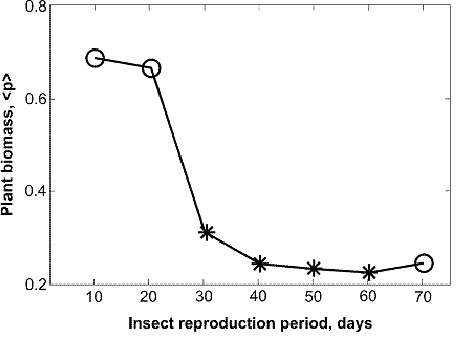 Research Example 11: Dependence
of the averaged plant biomass as a
function of insect production rates; O
= oscillations, * = chaos. Simulation
parameters roughly correspond to the
length of a normal growing season.
From Medvinsky, A. (2009). Chaos and
predictability in population dynamics.
NDPLS, 13(3), 311-326.
|
Nonlinear Dynamics in Education. Special issue of NDPLS (January, 2014) examines parent-child interactions from a dynamical point of view. See Contents. Special order this issue.
|
Applications - Education
|
|
|
Applications in education cover a range of individual-level, group-level, and institutional level topics. Examples include student learning and motivation dynamics, social dynamics in the classroom or school, student-teacher interactions, career development, absenteeism, and the long-run effect of policy concepts on the success of metropolitan school systems. There is some parallel between the topics addressed as education issues and those in organizational behavior more generally.
|
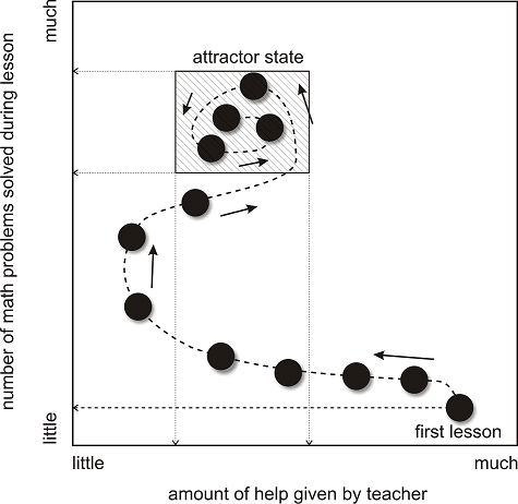 Research Example 12: A state space
describing the dimensions 'help given
by the teacher' and 'number of math
problems solved during one lesson
by the student,' together forming a
dynamic system. During the first lesson
the student is given much help and
solves only a few problems. Eventually
the system settles into an attractor
state. From Steenbeek, H., & van Geert,
P. (2013). The emergence of learningteaching
trajectories in education: A
complex dynamic systems approach.
NDPLS, 17(2), 233-268.
|
 Nonlinear Dynamical Systems
Analysis for the Behavioral
Sciences Using Real Data, edited
by Stephen J. Guastello and
Robert A. M. Gregson (2011).
Book covers a wide range of
traditional and statistically based
techniques for nonlinear
analysis, examples, experimental
design tips, and software
operation. See description.
Tutorials in Contemporary
Nonlinear Methods for the
Behavioral Sciences, edited by
M. A. Riley & G. C. Van Orden
(2005). A Digital Publication.
TISEAN Nonlinear Time Series
Analysis Routines by H. Kanz
& T. Schreiber. This widely
used program computes
correlation dimensions and
other traditional metrics from
real data after applying a
nonlinear filering routime for
error variance. Free donwload,
written in C).
Time Series Data Sources. We
put together a list of resources
where you can time freely
available time series data in
economics, physiology, etc.
|
An Overview of Nonlinear Methods
|
|
|
This section is compiled for the benefit of researchers who are
considering how they might start a project and organize their data
analysis. The first step is to conceptualize the formal dynamics that could apply to a problem and build a substantive theory in which psychological or other qualitative variables contribute to the dynamics. The model should be testable. Analytic strategies that have been developed to make computations that inform about the dynamics occurring in a data set include: the fractal dimension, Hurst exponent, Lyapunov exponent, BDS statistic, several measures of entropy, analyses based on polynomial regression or nonlinear regression, Markov chains, and symbolic dynamics. There are also visualization techniques such as phase space analysis, state-space grids, and recursion plots that have means for quantifying dynamics and various properties of the time series.
A strong theory about the phenomenon would greatly reduce
the number of models that should be tested. By the same token,
there is no reason to believe that the theoretical models that
originated in mathematics would be observed in their idyllic forms
in real data. Noise is always a challenge. For instance, there were
some early disappointments when what was thought to be chaos
turned out to be noise generated by the laboratory equipment.
One remedy for noise is to filter the data first, then proceed with
the calculations of choice results. By 'direct calculations' we mean
some computations that researchers have found meaningful early on were not statistical in nature, meaning that they assumed no further error in the data, did not rely on probability functions, and did not provide inferential tests of hypotheses. Statistical procedures for capturing the same underlying constructs were soon introduced. The strategy is that a nonlinear model,
chaotic or otherwise, needs to be tested statistically and separated
from residual variance. Filtering is sometimes possible as
when laboratory is corrected for AC hum. Noise can be introduced, however,
from all sorts of uncontrolled sources - uncontrolled events in
the laboratory experiments, uncontrolled individual differences
in responses to the experimental conditions, and measurement
error. In the classical measurement theory that social scientists usually rely upon, the measurement error (or noise) in a static distribution of observations is independent of any other errors and independent of the underlying true score or measurement. When the measurement is observed over time, however, the error subdivides into the classic form of error, which is now called independently and identically distributed (IID) error, and dependent error. Dependent errors interact with the true scores and other errors over time. The presence of dependent error is one hallmark of a nonlinear function.
The researcher then employs a statistical analyses, such as
polynomial regression or nonlinear regression, evaluate the
degree of fit between the model and data. The remaining variance unaccounted for is error, although it might offer some clues regarding how a modified model could be better. Note that there is
an assumption here that noise and 'true measurements' are
inseparable in raw form, and the goal of the analysis is to separate
the two portions of variance.
Transient effects are complications that occur in the dynamics
themselves. When transient effects occur, the dynamics change
for a period of time, and sometimes revert to the original dynamic
pattern. Transients can be difficult to identify and separate from the
core dynamic if the data sets are relatively short, which they often
are. The advisement to researchers is to look for a rule by which
the dynamics switch from one model to another, or from the core
dynamic to a [generic] transient and back again.
That said, we can provide an overview of the analyses that have had
the largest impact. The analyses can be divided between traditional
deterministically-based procedures. The traditional methods include phase space analysis, the
correlation dimension, and the Lyapunov exponent. The
stochastically-based procedures, which are often more compatible
with problems in the social sciences, include statistical analysis
for catastrophe models, redefinitions of the Lyapunov exponent
and correlation dimension for statistical analysis, some advanced
strategies for phase space analysis, and Markov Chain analysis.
Recursion Quantification Analysis (RQA), state space grids, symbolic dynamics
techniques, and entropy
statistics fall somewhere between the two camps.
|
|
Phase Space Analysis
|
|
|
A phase space diagram is a picture of a dynamical process that
can tell us quite a bit about the behavior of a system that follows
a particular function. It is usually drawn as a plot of the change
in X (DX) at time t+1 as a function of X at time t - velocity versus
position. The figures shown earlier for the fixed point, limit cycle,
and Lorenz attractors are phase space diagrams. There are a couple
other varieties of phase space diagram such as the return map,
which is a plot of X at time t+1 (rather than DX) as a function of X
at time t, and plots of two variables that are part of a more complex
function that involves two order parameters. Phase space diagrams
are useful tools for visualizing the dynamics inherent in a data set.
They are usually supplemented with metrics such as the correlation
dimension or Lyapunov exponent. It can be challenging to produce phase space diagrams for real
data because they do not provide any inferential statistics by
themselves, and the appearance of the diagram can be seriously affected by noise and by projecting the time series in an inadequate number of spatial
dimensions. Problems of spatial projection are generally
handled through analyses such as false
nearest neighbors or principal components analysis.
|
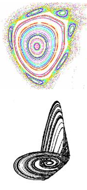 Phase space diagrams for two chaotic
attractors: The Henon-Hiles (upper), and
the Rossler (lower). Color is often used
to capture a fourth dimension of the
attractor.
|
|
Correlation Dimension
|
|||||||||||||||||||
|
Three descriptive metrics that are commonly applied to a time
series are the correlation dimension, the Lyapunov exponent, and
the Hurst exponent. The correlation dimension is a computation of
a fractal dimension. The basis of the algorithm is to take the time
series, treat it as a complicated line graph, and cover the graph with
circles of radius r. It then counts the number of circles required, then changes
the radius and repeats many times. Then it correlates the log of the
number of circles required with the log of the radius. The result will
be a line with a negative slope. The absolute value of the slope is
the fractal dimension.
Another popular calculation, involves the use of an embedding dimension,
which is described in the section on fractals appearing earlier. The correlation dimension is computed first with the assumption of an embedding dimension of 1, then assuming 2 dimensions, then 3, and so on. The computed fractal dimension will increase along with the embedding dimension up to a point where it reaching an asymptote, which is the final answer. The Grassberger-Procaccia algorithm is usually used for this purpose
and is included in the TISEAN and other software packages. The fractal dimension can
also be rendered by statistical means, which are described in a later
section of this page.
As mentioned earlier (and see the various links), fractal dimensions
characterize many structures of living and physical systems. They are
fractional taking on values in between the integer values associated with elementary geometry. Table 1 contains some rough interpretations.
Interpretation of Correlation
Dimensions
|
|
Surrogate Data Analysis and Experiments
|
|
|
The presence of fractal structure, if it is calculated through a
non-statistical method, is usually contrasted against an alternative interpretation, which
is that the fractal value for the time series could occur by chance. A statistical test of this
proposition can be performed as follows: (a) Take the time series
and randomly shuffle all the points. This process will preserve
the overall mean and standard deviation of the time series, but
will disrupt any serial dependency among the points if it exists.
(b) Repeat the shuffle 10, 100, 1000 times. (c) Calculate a fractal
dimension on each of the shuffled time series, and calculate the
mean and standard deviation of each of the fractal dimensions that
are obtained. (d) What are the odds that the fractal dimension that
was obtained from a true nonlinear function and not from the distribution
of values obtained from the shuffled time series?
Another way to finesse the noise problem is to conduct an
experiment in which something that is thought to affect the
complexity of the time series is systematically varied. In an
experiment, one might have separate groups of human subjects
that are performing a task under different conditions, and each
subject is producing a time series. Calculate the correlation
dimension for each subject, then compare the groups using a t-test,
analysis of variance, or similar type of analysis for an experiment. Non-parametric statistics are often preferred,
however. Any distortions in the nonlinear metric that were caused by error, noise, or sampling are
assumed to be equal or varying randomly across the experimental
conditions, and the mean differences in metrics such as the fractal dimension, entropy, etc. are what matter.
|
|
Lyapunov Exponent
|
|
|
The Lyapunov exponent evaluates the relative amount of expansion
and contraction between successive pairs of points in a time series.
It is perhaps best interpreted as a measure of turbulence in a
physical process or time series data.
As mentioned previously, it is actually a spectrum of values (when
calculated through the direct, or nonstatistical method). If the
largest value is a positive number, the series is chaotic. If the largest
value is negative, the series is contracting to a fixed point. Values
of 0 indicate either a straight line or a perfect oscillator. The nonstatistical
algorithms for the Lyapunov exponent are also susceptible
to distortions induced by noise. Once again surrogate data analysis
or statistically-based procedures can alleviate this problem.
The largest Lyapunov exponent,  , once obtained, can be converted
to a fractal dimension via the Kaplan-Yorke Conjecture: DL = e , once obtained, can be converted
to a fractal dimension via the Kaplan-Yorke Conjecture: DL = e .
Fractal dimensions (DL) calculated in this fashion should more
precisely identified as Lyapunov dimensions to distinguish the
algorithm used to produce it. .
Fractal dimensions (DL) calculated in this fashion should more
precisely identified as Lyapunov dimensions to distinguish the
algorithm used to produce it.
|
 Turbulent air flow. Produced and photographed
by Candace Wark and Shirley
Nannini. For more information, see their
article 'Cover images: Flow visualization,'
NDPLS, 21(1), 113-116.
|
|
The Hurst Exponent
|
|
|
The Hurst exponent, H, was first devised as a means of determining
the stability of water levels in the Nile River. Water flows in and flows
out, but is the net water level relatively stable or does it oscillate? To
answer this question, a time series variable, X with T observations is
broken into several subseries of length n; n is arbitrary. Then for each
subseries, the grand mean is subtracted from X, and the differences
summed. The range, R, is the difference between the maximum and
minimum values of the local means. Then rescaled range, R/s = (  *n/
2)H, where s is the standard deviation of the entire series; 0 < H <
1. Actual values of H may vary somewhat due to the choice of n and
the time scale represented by the individual observations.
A value of H = 0.5 represents Brownian motion, meaning that
the deflections in a time series can be upward or downward with
equal probability on each step. Brownian motion has a Gaussian
distribution and is non-stationary. Values that diverge from 0.5 in
either direction are non-Markovian, meaning that there is memory in
the system beyond the first step prior to an observation.
H > 0.5 denotes persistence. Deflections in a time series gravitate
toward a fixed point if H is high enough. The autocorrelation of
observations in a time series is positive. Values in the neighborhood
of 0.75 represent pink noise or self-organizing systems. H < 0.5
denotes anti-persistence; upward motions are followed by downward
motions, and the autocorrelation is negative.
In spite of the official range of H lying between 0 and 1, negative
values have been recently reported. The negative values arose
from the presence of a bifurcation in the data. It does not follow,
however, that all instances of bifurcations, such as those found in
catastrophe models, will always produce negative H values for a
time series. Further research is required on this matter. *n/
2)H, where s is the standard deviation of the entire series; 0 < H <
1. Actual values of H may vary somewhat due to the choice of n and
the time scale represented by the individual observations.
A value of H = 0.5 represents Brownian motion, meaning that
the deflections in a time series can be upward or downward with
equal probability on each step. Brownian motion has a Gaussian
distribution and is non-stationary. Values that diverge from 0.5 in
either direction are non-Markovian, meaning that there is memory in
the system beyond the first step prior to an observation.
H > 0.5 denotes persistence. Deflections in a time series gravitate
toward a fixed point if H is high enough. The autocorrelation of
observations in a time series is positive. Values in the neighborhood
of 0.75 represent pink noise or self-organizing systems. H < 0.5
denotes anti-persistence; upward motions are followed by downward
motions, and the autocorrelation is negative.
In spite of the official range of H lying between 0 and 1, negative
values have been recently reported. The negative values arose
from the presence of a bifurcation in the data. It does not follow,
however, that all instances of bifurcations, such as those found in
catastrophe models, will always produce negative H values for a
time series. Further research is required on this matter.
|
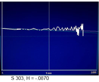 Research Example 13: This time series
for a cognitive task, which was performed
under conditions of fatigue,
displayed a negative Hurst exponent.
From: Guastello, S. J., Reiter, K., Shircel,
A., Timm, P., Malon, M., & Fabisch, M.
(2014). The performance-variability
paradox, financial decision making,
and the curious case of negative Hurst
exponents. NDPLS, 18, 297-328.
|
|
State Space Grids
|
|
|
The state space grid is a technique and computational program developed by Tom Hollenstein
for identifying attractor structures in experiments with real data.
As such, it is a useful alternative to the phase diagram when it is
not possible to deploy algorithms that involve multidimensional
projections of data.
The application starts with two variables that consist of ordered
categories. For instance, mother might behave in any of several ways, and the
child have any of several responses. Each observation consists of a point
that denotes the mother-child combination. The algorithm connects
the dots in time series. The algorithm then identifies the cells that
are most dense and can be interpreted as attractors. One can then
conduct experiments comparing theoretically interesting conditions and make statistical associations between the number and type of
attractors in the study.
|
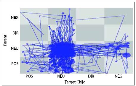 Research Example 14: An example
of a state space grid depicting a highentropy
and high conflict relationship,
from Dishion, T. J., Forgatch, M., Van
Ryzin, M., & Winter, C. (2012). Nonlinear
dynamics of family problem solving in
adolescence: The predictive validity of a
peacheful resolution attractor. NDPLS,
16(3), 331-352.
|
|
Recurrence Plots and Analysis
|
|
|
Although chaotic functions are said to produce non-repeating
patterns, repeatability is really a matter of degree. Visualizing what
repeats and how often can provide new insights to dynamics of
a process. A recurrence plot starts with a time series. The user
specifies a radius of values that are considered to be similar enough
and a time lag between observations that should be plotted. If a
the same value of X(t) appears after one or more lag units, a point in plotted. The
variable itself appears on the diagonal.
White noise would produce
a plot containing a relatively solid array of dots with no patterning. An oscillator would produce diagonal stripes. More interesting
deterministic functions would produce patterns; an example
pattern appears at the right. One can then calculate metrics that
distinguish one pattern from another such as the percentage of
total recurrences arising from the deterministic process, percentage
of consecutive recurrences, and the maximum length of the longest
diagonal (shorter is more chaotic).
Recurrence plots were first introduced as a procedure to accompany phase space analysis. New metrics, such as percent determinism,
were eventually introduced, and the name of the technique morphed
into recurrence quantification analysis (RQA). The new metrics were
valuable for interpreting a time series. Importantly RQA analysis
does not need to be accompanied by phase space analysis or assumptions about embedding versus fractal dimensions for proper interpretation.
A variation on the concept is to use plots of data from two different
sources (people) on the two axes instead of one source at two
points in time. This cross-recurrence technique has been used as
one method for studying synchronization phenomena.
|
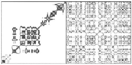 Research Example 15: Recurrence plot
for real (left) and reshuffled (right) data.
From Sabelli, H. (2001). Novelty, a measure
of creative organization in natural
and mathematical time series. NDPLS,
5(2), 89-114.
|
|
Nonlinear Statistical Theory
|
|
|
There is another genre of analysis that starts with a relatively firm
hypothesis that a particular nonlinear function is inherent in the
data. The function could be chaotic or reflect other types of dynamics. In the particular case of chaotic data,
the objective is to separate chaos from noise, just as one would
separate a linear trend from noise in a conventional regression analysis.
Consistent with four goals of inferential statistics, the regression-based analyses
can predict points, identify the nonlinear dynamics in
the data, report a measure of effect size, and determine statistical
significance of the parts of the respective models. The next
subsections of this exposition address issues concerning probability
density functions, the structure of behavioral measurements,
stationarity of time series, and what can be done to serve the
ultimate objectives.
Students of the late 20th century behavioral
sciences were taught to divide their probability distributions into
four categories: normal (Gaussian) distributions, those that would
be normal when the sample sizes became larger, those that would
be normal if transformations were employed, and those that were
so aberrant that non-parametric statistics were the only cure. In
the NDS paradigm, however, one is encouraged to assume specific
alternative distributions such as power law, exponential, and
complex exponential distributions. To take things a step further, any
differential function can be rendered as a unique distribution in the
exponential family, and the presence of an exponential distributions
or a power law distribution in a time series variable denotes a
nonlinear function contained therein.
Dependent error in a dynamical process, which was introduced earlier, might occur like this:
Imagine we have a measurement that is iterating through a process
such that X2 = f(X1). The function produces X3, X4, etc. the same way.
Now let a random shock of some sort intrude at X4. At the moment
the shock arrives, the error is IID. At the next iteration, however, X5 =
f(X4 + e); the error continues to iterate with the true score through
the ensuing time series.
Other ways for dependent error to occur are when errors are
autocorrelated or when complex lag effects are in play such that
X(t) = f[X(t-1), X(t-3)]. Fortunately there is a proof due to William
Brock and colleagues showing that the presence of dependent error
in the residuals of a linear autocorrelation is a positive indicator
of nonlinearity. Furthermore, if a good-enough nonlinear function is specified
for the true score, the dependent error is reduced to a minimum.
So, what does it take to specify a good-enough nonlinear function?
Researchers should have the dynamics for their theory worked
out in sufficient detail. To do so requires study of the extant
literature on the particular application.
Fortunately there are some groups of options that have some
degrees of flexibility. Consider two examples:
Example 1:  z = b0 + b1z13 + b2Bz1 + b3A
Example 2: z2 = z = b0 + b1z13 + b2Bz1 + b3A
Example 2: z2 =  1Bz1*exp( 1Bz1*exp( 2z1) + 2z1) +  3
where z is the dependent variable (order parameter) that is
measured at two or more points in time, 3
where z is the dependent variable (order parameter) that is
measured at two or more points in time,  z is a change in the
dependent variable, A and B are control (independent) variables,
bi are linear regression weights, and z is a change in the
dependent variable, A and B are control (independent) variables,
bi are linear regression weights, and  i are nonlinear regression
weights. For models similar to Examples 1 and 2, data are prepared
by setting a zero point and a standard calibration of scale for all
variables in the model. Thus the dependent variable is represented
by z instead of the conventional X or Y.
Any error associated with approximating a differential function from
a difference function becomes part of [1- R2]. The use of R2 in this
context is predicated on the use of least squares statistical analysis,
which is an effective and very reasonable approach to nonlinear
statistical analysis.
Example 1 is a cusp catastrophe executed with ordinary polynomial
regression. Example 2 is part of a series of exponential models
developed by Stephen Guastello that is executed through nonlinear
regression. In Example 2, i are nonlinear regression
weights. For models similar to Examples 1 and 2, data are prepared
by setting a zero point and a standard calibration of scale for all
variables in the model. Thus the dependent variable is represented
by z instead of the conventional X or Y.
Any error associated with approximating a differential function from
a difference function becomes part of [1- R2]. The use of R2 in this
context is predicated on the use of least squares statistical analysis,
which is an effective and very reasonable approach to nonlinear
statistical analysis.
Example 1 is a cusp catastrophe executed with ordinary polynomial
regression. Example 2 is part of a series of exponential models
developed by Stephen Guastello that is executed through nonlinear
regression. In Example 2,  2 corresponds to the largest Lyapunov
exponent; if 2 corresponds to the largest Lyapunov
exponent; if  2 is positive and 2 is positive and  3, the constant, is negative, then
both expanding and contracting properties exist in the data set.
Expanding and contracting trajectories denote chaos. It is also possible to
expand the model by substituting a second exponential function
for 3, the constant, is negative, then
both expanding and contracting properties exist in the data set.
Expanding and contracting trajectories denote chaos. It is also possible to
expand the model by substituting a second exponential function
for  3. There is also a series of model structures for determining
oscillators and coupled oscillators that was developed by Steven
Boker, Jonathan Butner and colleagues; the essential concepts of
nonlinear time series analysis apply to these structures as well.
The results of the nonlinear models should be compared against
alternative theoretical models. The researcher is looking for a higher
degree of fit between the model and the data compared to the
alternatives, and all the parts of the nonlinear model should be
supported as well. The alternatives are often linear but not always
so. 3. There is also a series of model structures for determining
oscillators and coupled oscillators that was developed by Steven
Boker, Jonathan Butner and colleagues; the essential concepts of
nonlinear time series analysis apply to these structures as well.
The results of the nonlinear models should be compared against
alternative theoretical models. The researcher is looking for a higher
degree of fit between the model and the data compared to the
alternatives, and all the parts of the nonlinear model should be
supported as well. The alternatives are often linear but not always
so.
|
|
Maximum Likelihood Methods
|
|
|
Jonathan Butner and colleagues have been experimenting with new
adaptations of growth mixture modeling, multilevel modeling, and
latent class analyses for identifying dynamics in data. The essential
problem that they are addressing is that one might have no clue
(hypothesis) in advance as to what combinations of attractors, bifurcations,
or saddles, might be lurking in the data. The
first two diagrams at the right are time series plots of two variables
in a system they were studying. The third is a vector and density
plot of the two variables.
|
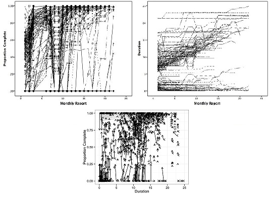 Research Example 16: Time series for
two system variables (upper),
and a vector-and-density plot of the two
variables (lower). From Wiltshire, T. J., Butner, J.
E., & Pirtle, Z. (2017). Modeling change
in project duraction and completion:
scheduling dyanmics of NASA's Exploration
Flight Test 1 (EFT-1) activities. NDPLS,
21(3), 335-358.
|
|
Markov Chains
|
|
|
The concept of Markov chains originated outside the realm
of nonlinear science. The central idea is that the researcher is
observing objects or people in a finite set of possible states. Objects
all have odds of moving from one state to another. The State X
State matrix of odds is a transition matrix. The analysis establishes the transition matrices and determines the
arrival of objects into states. Stephen Merrill illustrated that some combinations of transitions could result in fixed points,
oscillators, bifurcations, or chaotic outcomes. Thus Markov chain
analysis now falls into the scope of nonlinear dynamical analyses.
There is also a subtle connection between Markov chain analyses
and the methods of symbolic dynamics that have been deployed for
real data in the behavioral sciences thus far.
|
|
Symbolic Dynamics
|
|
|
Symbolic dynamics is an area of mathematics that finds patterns
in series of qualitative data. The elementary patterns themselves
can be treated like qualitative states and analyzed for higher order
patterns. This class of techniques is ideally suited to analyzing
chaotic and related complex nonlinear dynamics, either in the
form of continuously valued time series or qualitative categorical data. Symbolic dynamics are particularity useful in situations in which discontinuities, continuities, periodic functions, and unnamable
transients could co-exist within a relatively short time series. For
continuous data, events such as spikes and small or large up-trends
and down-trends are coded nominally (e.g., with letter codes A, B,
C, D, etc.) and then analyzed. For categorical data, the categories, which should be theoretically relevant, are also given letter codes, and the
computations are carried out essentially the same way. The techniques that are available vary in their means for
determining symbol sequences and the length of those sequences.
Orbital Decomposition (ORBDE) analysis, which was developed by Stephen Guastello and colleagues, can disentangle periodic patterns that contribute to a globally chaotic time series. It is particularly good for empirically determining the optimal pattern length. It includes entropy metrics and tests for determining the extent to which the patterns that were isolated by the analysis deviate from chance levels of occurrence. In this way it can distinguish between chaotic and random sequences.
Topological entropy is the primary entropy metric used for determining pattern
length. It approximates the Lyapunov
exponent under limiting conditions. Unlike Shannon entropy, which
is also reported in the analysis, the topological entropy metric preserves the
temporal sequence of the events that are being extracted.
The ORBDE software is available from the link at the left. The
current version (2.4) allows analysis for multiple categorical variables to
be evaluated simultaneously. One can also apply varying numbers
of codes to a single event. For instance, a short utterance
in a conversation between two or more people might have only one
category of content (e.g. asking a question), but a longer utterance
might contain several categories of content. Komolgorov-Sinai
entropy, which is an expansion of Shannon entropy, is calculated for
the multiple-variable analyses.
|
